Monitoring the Environment and Biodiversity

Why Monitor Ecosystems?

Scientists monitor the distribution and abundance of organisms to understand the health of ecosystems and detect the effects of human activity or environmental change. Field investigations use sampling techniques to estimate population sizes without counting every individual — a practical necessity when populations are too large or too mobile to census directly. This type of fieldwork is a key skill in biology practical work (PAG B3).

Sampling Techniques

Random sampling uses quadrats placed at coordinates generated randomly (e.g. using a random number table) to avoid bias. The researcher has no influence over where quadrats land. This is suitable for slow-moving or stationary organisms such as plants, limpets or ground-dwelling invertebrates. Results from multiple quadrats are averaged and scaled up to estimate total population size.

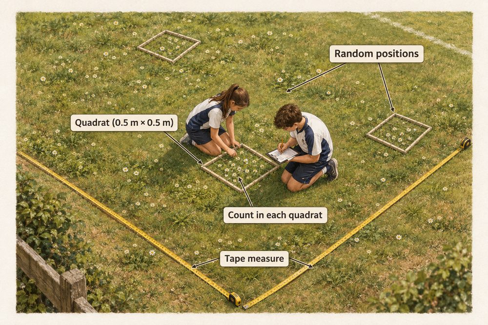
Diagram: To estimate a population, scientists place quadrats at random positions, count the organisms in each and work out a mean.

Transect sampling places quadrats or records organisms at regular intervals along a line called a transect. This is used to investigate how species distribution changes across a habitat in response to changing abiotic conditions — for example, from the low shore to the high shore of a rocky beach, or from open grassland into a woodland. A belt transect records all organisms within a strip on either side of the line; a line transect records only organisms touching the line.

Key Fact

Random quadrat sampling avoids bias and suits stationary organisms. Transect sampling shows how species distribution changes across a habitat in response to abiotic gradients. Capture-recapture estimates mobile animal populations.

Capture-Recapture and the Lincoln Index

Mobile animals cannot be counted using quadrats. The capture-recapture method involves catching a sample of animals, marking them (e.g. with paint, tags or notches), releasing them, and later catching a second sample. The proportion of marked individuals in the second sample allows the total population size to be estimated using the Lincoln Index:

$$N = \frac{n_1 \times n_2}{m_2}$$

Where $N$ = estimated population size, $n_1$ = number in first sample, $n_2$ = number in second sample, $m_2$ = number of marked individuals in the second sample.

For example: 40 woodlice are caught, marked and released ($n_1 = 40$). The next day, 35 are caught ($n_2 = 35$), of which 7 are marked ($m_2 = 7$).

$$N = \frac{40 \times 35}{7} = \frac{1400}{7} = 200$$

The estimated population is 200 woodlice. The accuracy of this estimate depends on several assumptions: marked individuals must mix randomly back into the population; marking must not affect survival, behaviour or attractiveness to predators; the population must be closed (no significant births, deaths, immigration or emigration) between the two samples. If these assumptions are violated, the estimate will be unreliable.

Indicator species reveal pollution levels without expensive instruments. Lichens are sensitive to sulfur dioxide in the air: bushy, leafy lichens grow only in clean air, while crusty lichens tolerate some pollution. Their absence indicates heavily polluted air. Freshwater invertebrates indicate water quality. Stonefly nymphs and freshwater shrimps require clean, well-oxygenated water; their presence indicates low pollution. In contrast, bloodworms (Chironomus larvae) and rat-tailed maggots tolerate low-oxygen, polluted water. A healthy, diverse community of invertebrates suggests good water quality.

Scientists also take direct physical measurements to confirm what indicator species suggest: dissolved oxygen meters, pH probes and nitrate test kits provide quantitative data. Combining biological and physical indicators gives a fuller picture of ecosystem health.

Biodiversity and Human Impact

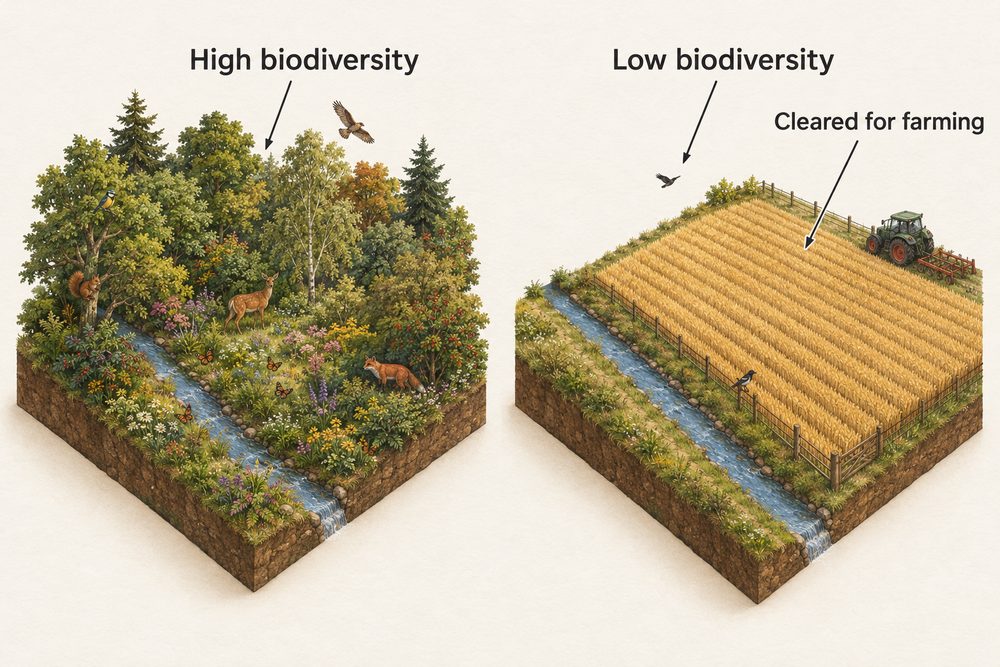
Biodiversity refers to the variety of living organisms in an area. High biodiversity indicates a healthy, stable ecosystem with many different species filling different ecological roles. Human activities reduce biodiversity through deforestation (habitat loss), pollution, over-exploitation of species and the introduction of invasive non-native species that outcompete native ones.

Diagram: The same piece of land as a varied woodland and after it is cleared for farming shows how human activity reduces biodiversity.

Eutrophication is a serious consequence of agricultural pollution. When excess nitrate or phosphate fertilisers wash into rivers and lakes, they trigger rapid algal growth (an algal bloom). Dense algae block sunlight, killing aquatic plants below. When algae die, decomposing bacteria multiply and consume dissolved oxygen. Oxygen levels fall so low that fish and other aerobic organisms suffocate. This sequence — nutrient enrichment, algal bloom, light blocking, decomposition, oxygen depletion — is a clear example of a negative human interaction with an ecosystem (B6.1b).

Sustainability requires managing ecosystems so that human use does not exceed natural recovery rates. Conservation strategies include:

• Protected areas — national parks and nature reserves limit harmful human activity.
• Captive breeding programmes — endangered species are bred in captivity with plans for reintroduction to the wild.
• Seed banks — storing seeds from rare plant species as insurance against extinction.
• Fishing quotas and logging regulations — controlling extraction rates to allow populations to recover.
• Reforestation — planting trees to restore habitats and sequester carbon dioxide.

Effective conservation requires long-term monitoring data to determine whether strategies are working, and cooperation between governments, local communities and scientists.